
WAMSIM

How to use WAMSIM
- When you click on the "WAMSIM" icon, the site for the genetic effect evaluation version of the WAM simulator(https://wamsim.vdslab.jp/)will open in a separate window.
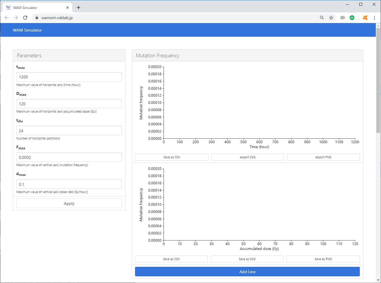
- Fill in the "Parameters" on the left hand side, and press the "Apply" button.
tmax : The maximum value for the x-axis "time exposed to radiation (Time (hours))", for the graph on the right hand side, as well as the two types of graph (Mutation Frequency and Dose Rate) displayed by the operation of "3.".
Dmax : The maximum value for the x-axis "total radiation dose (Accumulated Dose (Gy))", for the lower graph on the right hand side, as well as the lower graph of Mutation Frequency displayed by the operation of "3.".
tdiv : Number of minor tick marks on the x-axis - how many tmax values - to divide, for the upper graph on the right hand side, as well as the two types of graph (Mutation Frequency (upper) and Dose Rate) displayed by the operation of "3.".
Fmax : The maximum value of the Y-axis "Mutation Frequency", for the graph on the right hand side, as well as the the graph of Mutation Frequency displayed by the operation of "3.".
dmax : Maximum value of Y-axis "Dose rate (Gy / hour)" of the Dose Rate graph displayed by the operation of "3." - When you click the blue "Add Line" button at the bottom of the right hand graph, a graph for inputting the dose rate will display in the bottom of the window.
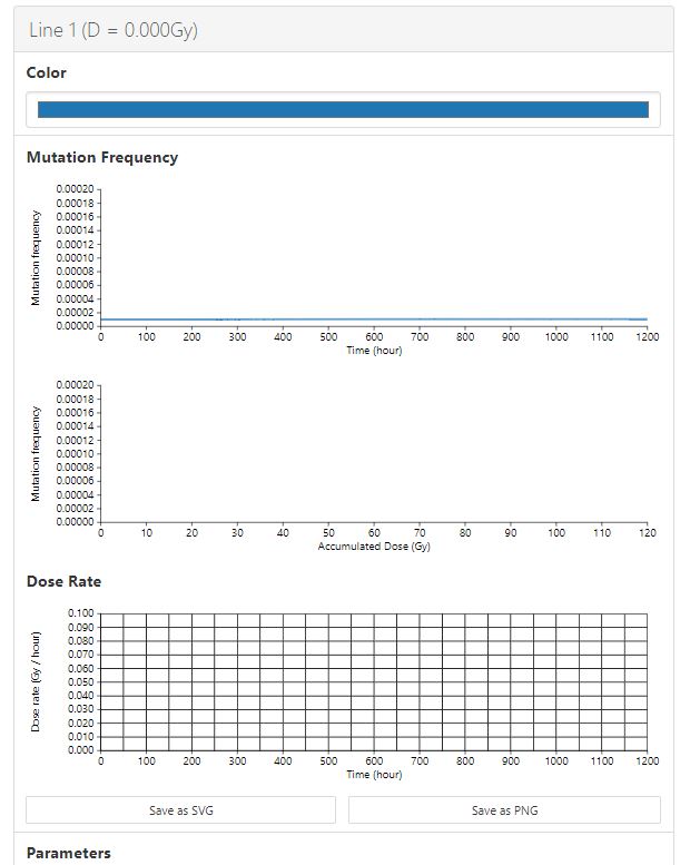
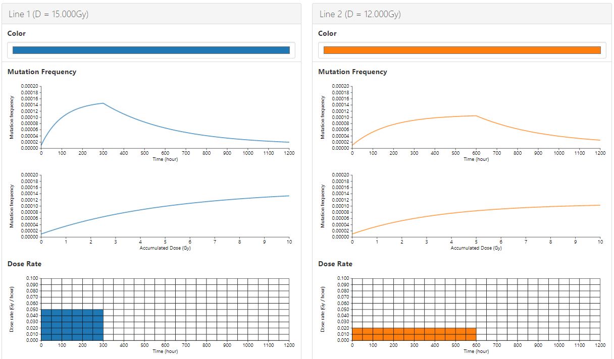
Color : Sets the color of the line to displayed on the graph.
Mutation Frequency : The results of the WAM Model calculations will be displayed here once you have set the dose rate below.
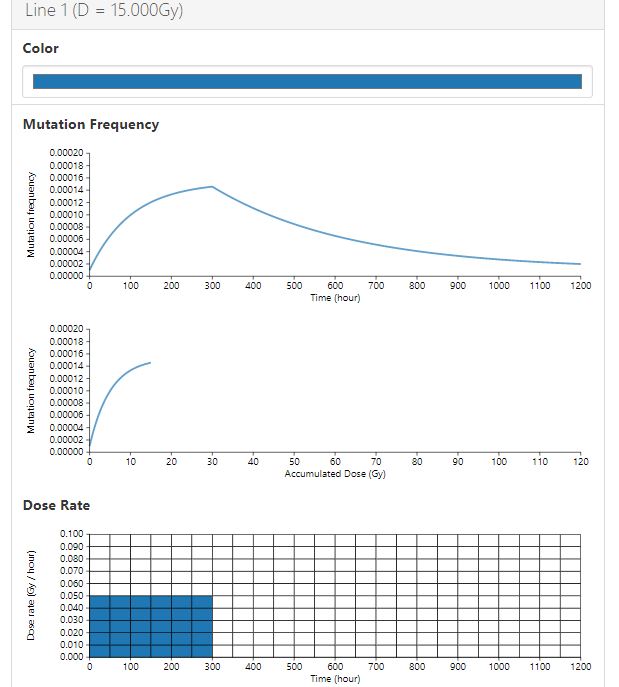
Dose Rate : Sets the irradiation time (hour), irradiation schedule, and dose rate (Gy/hour) (see "5.").
Parameters :These are the parameters(*) the WAM model uses in its calculations.
* This defaults to the parameter set for mice estimated from the experimental values of the mouse-genetics program from the ORNL (Oak Ridge National Laboratory) by the William L. Russel Research Group. - Adjust the values of each parameter using the sliders.
(As these values can be adjusted even after drawing the graph, use the default values when using the simulator for the first time.) - You can adjust the irradiation time (hour), irradiation schedule, and dose rate (Gy/hour) using your mouse under the "Dose Rate" graph.
If you input these values using the mouse, the "Mutation Frequency" graph will immediately redraw the result of calculations.
- If you need to compare the results of multiple calculations, repeat the procedure in steps"3."-"5.".
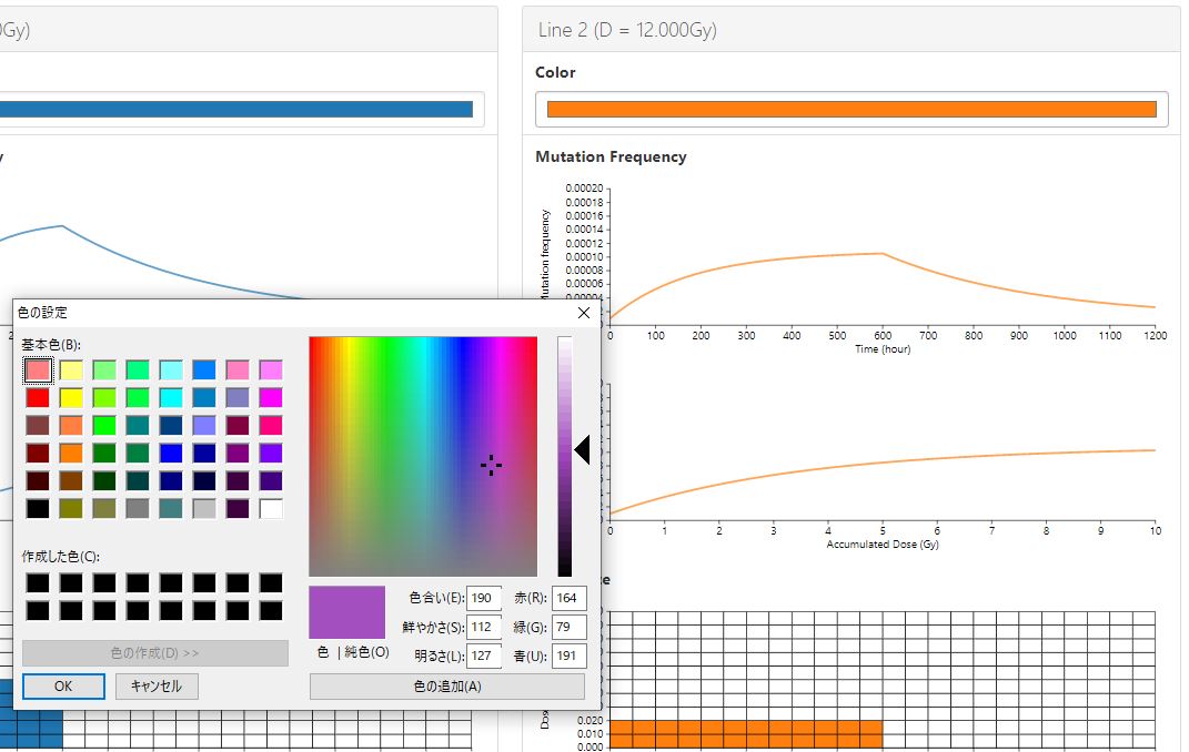
- If you would like to change the color of the graph lines, click the "Color" button and choose the color you want.
- For the results of multiple calculations, the lines will be drawn on top of each other in the "Mutation Frequency" graph in the top right of the page.
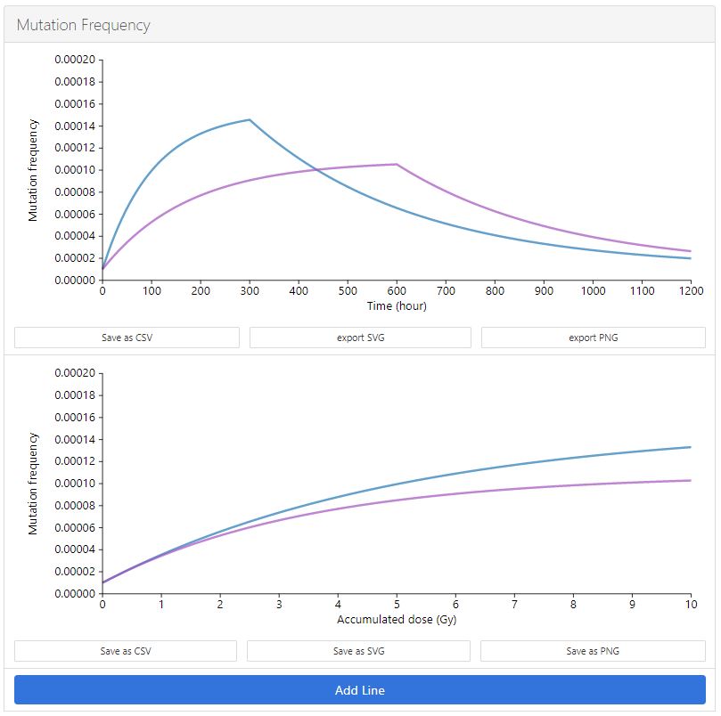
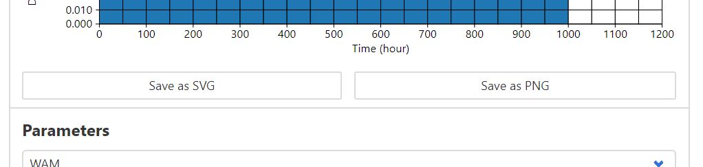
- If you need to export and save the "Mutation Frequency" graph, click the "Export ***" and/or "Save as ***" icons.
Save as CSV : exports text data (in the form of a .csv file
export SVG, Save as SVG : exports vector data (in the form of a .svg file)
export PNG, Save as PNG : export PNG: exports bitmap data (in the form of a .png file)
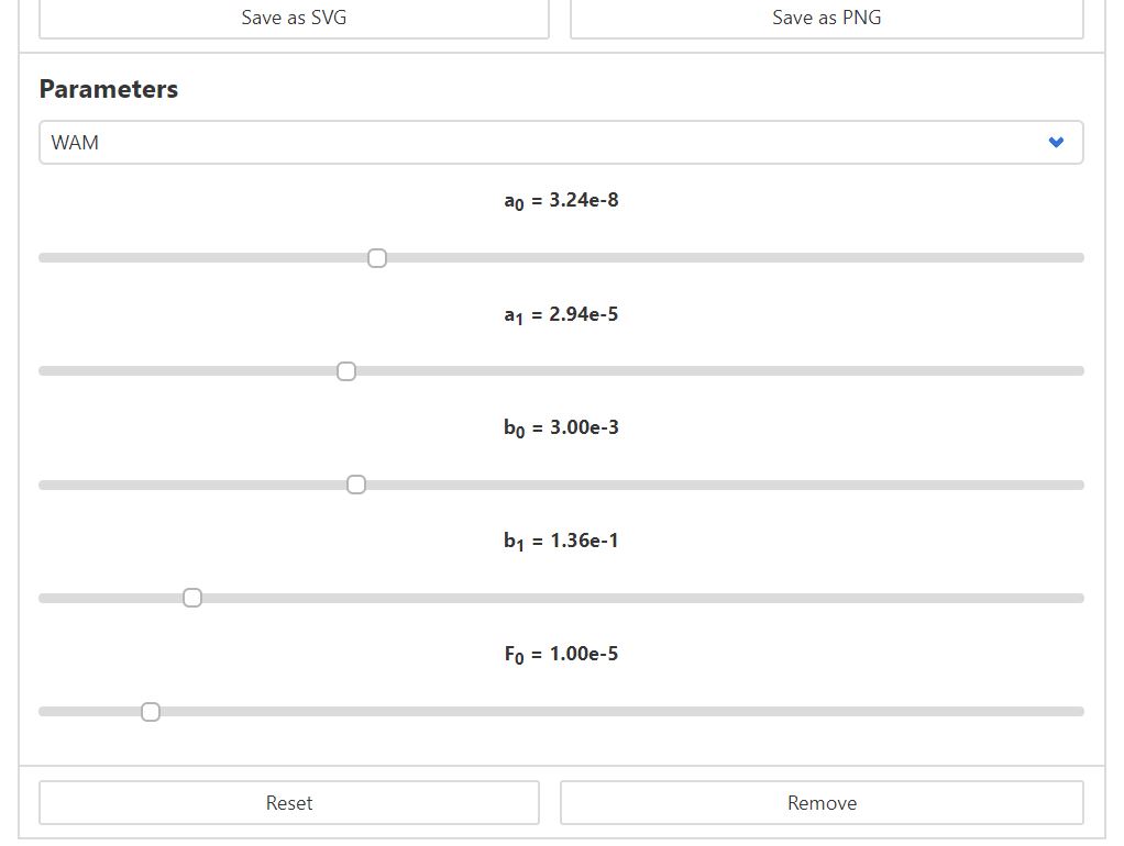
a0 : Increase and incidence of mutation occurring in the natural environment [/hour]
a1 : Increase and incidence of mutation due to additional radiation dosage. [/Gy]
b0 : Decrease in mutated cells due natural factors such as natural cell death [/hour]
b1 : Decrease in mutated cells due to cell death caused by radiation [/Gy]
F0 : Rate of natural spontaneous mutation.
The pull-down menu allows you to select how to calculate the mutation frequency.
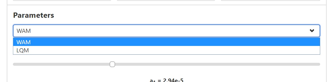
WAM : calculation by WAM model.
LQM : calculation by LQM (linear-quadratic model; conventional model).
Examples of WAMSIM in use
Here are a few examples of the model in action.
We have touched up the dose rate graph in order to make it easier to see. This will be filled in the actual WAMSIM.
All of these examples also use the default parameter set (in other words, they show what the model predicts for mice).
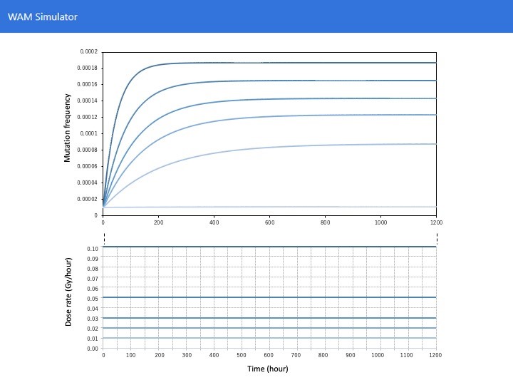
- Comparative results of the mutation frequency among surviving mice under different dosage rates.
Dosage rates of 0, 0.01, 0.02, 0.03, 0.05, and 0.10 Gy/hour of gamma radiation for 1200 continuous hours.
Dosage rates of 0, 0.01, 0.02, 0.03, 0.05, and 0.10 Gy/hour of gamma radiation for 1200 continuous hours. (0 Gy/hour represents the control with no damage from additional radiation, or, in other words, the background level of radiation).
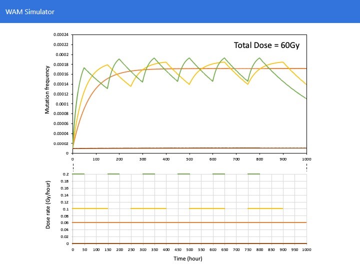
- Comparative results of the mutation frequency in the case of different numbers of exposures during fractionated irradiation.
0 Gy/hour is the control (i.e. before exposure).
Comparison of a total exposure dose of 60 Gy with an exposure dose 0.06 Gy/hour over 1,000 continuous hours, an exposure rate of 0.1 Gy/hour in four periods of 150 hours of continuous exposure, and an exposure rate of 0.2 Gy/hour over six periods of 50 hours of continuous exposure.
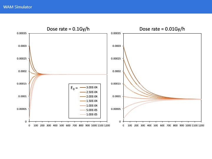
- Comparative results of the mutation frequency in the case of differing rates of natural mutation.
Under dose rates of 0.1 Gy/hour (left graph) and 0.01 Gy/hour (right graph) over 1,200 continuous hours, the F0 parameter is changed (the default value is 1.0e-05).
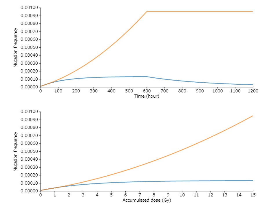
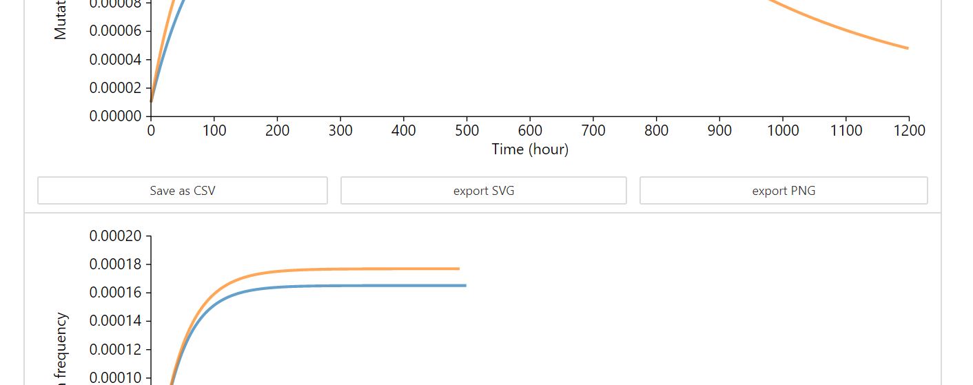
- Comparison of LQ model which have been widely used and WAM model.
Continuous irradiation (total irradiation dose 15 Gy) for 600 hours at a dose rate of 0.025 Gy/hour.
In the LQ model which does not consider the repair effect, the mutation frequency increases rapidly as the irradiation time passes, and does not decrease even after stopping the irradiation (even after 600 hours).